Multiyear tropical warm pool warming drives slowdown in Antarctic mass loss

Data

Ice mass variability was quantified using GRACE and GRACE-FO gravimetry data⁵⁰ spanning 2003–2024. SMB (precipitation minus meltwater runoff, sublimation, evaporation and wind erosion) outputs from RACMO2.4p1 (ref. ⁵¹) and MARv3.14 (refs. ^52,53) were used to link precipitation variability to observed ice mass changes. Precipitation variability was assessed using several independent datasets, including ERA5 (ref. ⁵⁴) and MERRA-2 (ref. ⁵⁵) reanalyses and RACMO2.4p1 regional climate-model precipitation, to ensure consistency across data sources. The Law Dome ice-core snow-accumulation record⁴⁹ was used as extra observational input. Large-scale circulation and moisture transport were analysed primarily using ERA5 fields, including SST, Z300, evaporation and integrated water vapour transport (IVT). Velocity potential was obtained from NCEP-NCAR Reanalysis 1. The Niño 3.4, IOD, IPO, zonal wave-3 and Southern Annular Mode⁵⁶ indices were used to examine their relationships with TWP variability. To assess the frequency of TWP warming events, we analysed both ERA5 (1950–2025) and the CESM1 Large Ensemble⁵⁷, including the 1,800-year fully coupled pre-industrial control simulation and the 40-member historical and RCP8.5 simulations. To provide an independent long record check of the TWP–East Antarctic dipole–QW precipitation relationship, we also used two paleo-reanalysis products. EKF400v2 (ref. ⁵⁸) provides monthly fields of Z500, 2-m air temperature and precipitation from 1603 to 2003. LMR v.2.1 (ref. ⁵⁹) provides last-millennium ensemble reanalysis fields of Z500, SST and precipitation on an annual basis. Because EKF400v2 does not provide SST, its 2-m air temperature field was used as an indicator of SST variability. Monthly anomalies were generally calculated by removing the climatological seasonal cycle.

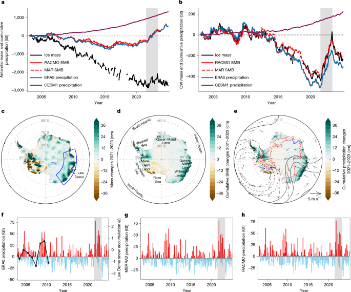
Guided by the spatial pattern of mass and cumulative precipitation anomalies, QW was defined as the region spanning 70–145° E and 65–75° S. The TWP was defined as a 15° clockwise-rotated ellipse centred at 135° E, 5° S, with semi-major and semi-minor axes of 35° and 15°, respectively, on the basis of the observed relationships between EA precipitation and tropical SSTs. We also defined an EA dipole index as the area-mean Z300 anomaly over the EA high-pressure centre (55°–70° S, 120°–160° E) minus that over the low-pressure centre south of Australia (30°–50° S, 80°–150° E).

Significance testing

Statistical significance of correlations, regressions and trends was assessed using two-tailed Student’s t-test at the 95% confidence level, with the effective sample size corrected for autocorrelation.

Here N is the total number of samples, and r₁ and r₂ are the lag-1 autocorrelation coefficients of the two correlated time series. For spatial fields, statistical significance was further controlled using false discovery rate correction⁶⁰.

MCA decomposition

MCA⁶¹ is a multivariate statistical technique that uses singular value decomposition on the cross-covariance matrix of two fields to extract paired spatial patterns and time series that maximize their covariance. Each MCA mode represents a linear combination of the original variables that captures a specific covarying structure shared by the two fields. The importance of each mode is measured by the squared covariance fraction, which indicates the proportion of total squared covariance explained by that mode. Higher squared covariance fraction values denote leading modes of coupled variability. In this study, MCA was applied to deseasonalized and detrended monthly anomalies of ERA5 Z300 south of 23° N and Antarctic precipitation for 1979–2024.

WAF diagnosis

Stationary Rossby-wave propagation was diagnosed using the Takaya and Nakamura⁶² WAF formulation. Horizontal WAF vectors (W) were computed from geopotential height anomalies relative to the climatological mean flow:

where ({psi }^{{prime} }) denotes the geostrophic streamfunction anomaly derived from the geopotential height (Z), defined as ({psi }^{{prime} }=g{Z}^{{prime} }/f) (where g is gravitational acceleration and f is the Coriolis parameter); U = (U, V) represents the climatological mean horizontal wind vector with a magnitude of (|{bf{U}}|=sqrt{{U}^{2}+{V}^{2}}). The coordinates are given by longitude (λ) and latitude (φ). In addition, a represents the Earth’s radius and p denotes the pressure level (normalized by 1,000 hPa).

AR detection

Monthly AR-frequency anomalies were regressed onto standardized MCA3 Z300 time series to diagnose their relationship with the dipole circulation. ARs were identified using the Guan and Waliser⁶³ detection algorithm. This updated and validated version is particularly suitable for high-latitude regions such as Antarctica, where background moisture is climatologically low. Its effectiveness in these regions is attributed to its use of season-dependent and location-dependent IVT thresholds, instead of a fixed global threshold, allowing for the robust identification of poleward moisture intrusions relative to the local background state.

The detection was applied to 6-hourly IVT fields derived from 6-hourly wind and specific humidity integrated from 1,000 hPa to 300 hPa:

where g is the gravitational acceleration, u and v are the zonal and meridional wind components and q is the specific humidity. The detection process involved three key criteria⁶³: (1) intensity threshold: the IVT magnitude had to exceed the 85th percentile of the local monthly IVT climatology, or 100 kg m⁻¹ s⁻¹, whichever was larger; (2) geometry: the detected filament had to have a length greater than 2,000 km and a length-to-width ratio greater than 2 and (3) directional coherence: the mean IVT direction had to be consistent to exclude moisture features without coherent poleward transport. Monthly AR frequency was calculated by averaging the daily occurrence counts within each month, with daily counts derived from the 6-hourly detections. We note that the Guan and Waliser⁶³ detection algorithm tends to sufficiently capture ARs over the Southern Ocean, but may be less effective at capturing ARs after landfall^34,37. We adopted it here because our analysis required a consistent AR detection method across the SH, rather than a regional algorithm.

Eddy vorticity budget diagnosis

To diagnose the dynamical processes responsible for the formation and maintenance of the meridional dipole between the southern Australian low and the EA high, we analysed the relative vorticity budget following the framework of ref. ⁶⁴. The relative vorticity tendency at a given pressure level is given by ref. ⁶⁵:

where ζ is relative vorticity, f is the Coriolis parameter, u = (u, v) is the horizontal wind vector, ω is vertical velocity in pressure coordinates and F represents frictional forcing.

Using standard scaling arguments⁶⁵, the vertical advection and tilting terms are at least one order of magnitude smaller than the horizontal vorticity flux convergence and are therefore neglected. Each variable is decomposed into a seasonal-mean component (denoted by an overbar) and an anomaly (denoted by a prime). The anomalous vorticity tendency equation can then be written as⁶⁴:

The first term represents vorticity generation by anomalous divergence and is referred to as the stretching term. The second term denotes the convergence of anomalous vorticity fluxes and is referred to as the eddy forcing term, which captures the dynamical feedback between transient eddies (periods shorter than 7 days) and the low-frequency circulation. The third term is the linear wave term, describing the advection of background vorticity by anomalous winds and advection of anomalous vorticity by the mean flow, and is associated with Rossby-wave propagation. The fourth term consists solely of climatological quantities and represents stationary-wave forcing; it varies weakly in time and was therefore not considered in the temporal correlation analysis.

Sensitivity experiments

To assess the role of TWP SST anomalies in driving the precipitation over EA, we conducted a suite of sensitivity experiments using two AGCMs⁶⁶, ECHAM5 and CAM5. The ECHAM5 model was run at T42 spectral resolution (roughly 2.8° × 2.8°) with 19 vertical levels extending to 10 hPa, following a standard AMIP-style configuration. A 40-year control simulation was first performed using monthly climatological SSTs and sea ice concentrations derived from ERA5 for 1979–2024. Greenhouse gas concentrations and aerosols were fixed at year-2000 levels, thereby excluding transient anthropogenic forcing.

A total of eight sensitivity experiments were conducted by superimposing prescribed SST anomalies onto the control SST climatology. Each experiment was integrated for 40 years, and the atmospheric response was defined as the difference between the sensitivity experiment and the control simulation. Experiment 1 imposed a positive SST anomaly over the TWP. The TWP region was defined as a 15° clockwise-rotated ellipse centred at 135° E, 5° S, with semi-major and semi-minor axes of 35° and 15°, respectively. Experiment 2 combined the TWP warming with a negative IOD-like cooling anomaly (ellipse centred at 65° E, 5° N; axes 30° × 15°) and a La Niña-like cooling anomaly over the eastern Pacific (ellipse centred at 130° W, 0° N; axes 60° × 15°). Experiments 3 and 4 were designed to isolate the effects of the cooling anomalies: experiment 3 was driven solely by the La Niña-like cooling in the eastern Pacific and experiment 4 was driven solely by the negative IOD cooling in the northwestern Indian Ocean. Experiment 5 was driven by positive SST anomalies over the SPCZ region (a 10° clockwise-rotated ellipse centred at 200° E, 25° S, with semi-major and semi-minor axes of 60° and 8°, respectively) to examine the impact of SPCZ-related warming. Experiment 6 examined the modulation by background warming by superimposing the TWP SST anomaly onto a uniform +0.5 K SST increase applied across the tropical band (30° S–30° N). Experiment 7 was identical to experiment 6 but intensified the TWP warming magnitude by an extra 0.5 K. Experiment 8 replicated the forcing configuration of experiment 1 but used the CAM5 model to verify the robustness of the results and rule out model dependence.

For standard warming or cooling scenarios (experiments 1–6 and 8), anomalies increased from ±0.5 K at the boundaries to a peak amplitude of ±1 K at the centre. For the strong TWP warming case (experiment 7), the anomaly ranged from 1 K at the edge to 1.5 K at the centre.

As observed in both the SST anomaly pattern associated with the MCA3 mode (Extended Data Fig. 5c) and the mean SST anomalies during 2021–2023 (Extended Data Fig. 2b), La Niña-like SST cooling, negative IOD cooling and SPCZ warming co-occurred with the prolonged TWP warming. When both cooling patterns were imposed alongside TWP warming (Experiment 2, Extended Data Fig. 8a), the Z300 response showed a more localized low-pressure anomaly over southern Australia and a more pronounced high-pressure anomaly centred north of the Ross Sea, accompanied by a precipitation response over EA comparable to that in experiment 1. By contrast, experiments 3–5, which isolated the La Niña-like cooling, IOD-like cooling and SPCZ warming, respectively (Extended Data Fig. 8b–d), failed to reproduce the significant EA dipole circulation pattern or positive precipitation anomalies near QW, suggesting that these three SST anomaly components were not the key forcings driving the observed response.

In a future warming world, tropical mean SSTs are expected to increase, as is evident in CESM1 future projections. The 30-year mean SST during 2021–2050 is warmer than that during 1991–2020 by about 0.5 K across nearly the entire tropics (not shown). How this background warming modulates the circulation response to TWP warming was illustrated with experiment 6, representing the occurrence of TWP anomalies within the warmer background state expected in the coming decades. Under this forcing, the Z300, surface temperature and precipitation responses over EA were notably less significant (Extended Data Fig. 8e). This attenuated response probably resulted from the uniform tropical warming reducing the relative SST gradient between the TWP and its surrounding regions, thereby damping the effective convective heating anomaly over the TWP. When the magnitude of the TWP warming was increased (experiment 7), the response over EA became pronounced again, aligning closely with the results of experiment 1 (Fig. 3 and Extended Data Fig. 8f). This indicates that the atmospheric circulation over EA is preferentially sensitive to the localized SST gradients driven by TWP warming, rather than to broad, basin-wide tropical warming.

Finally, experiment 8 repeated the experiment 1 forcing using CAM5, performed in the same AMIP-style framework at 1.9° × 2.5° horizontal resolution with 30 vertical levels, and reproduced a north–south dipole circulation pattern and enhanced precipitation over EA similar to those simulated by ECHAM5 (Extended Data Fig. 9), confirming that the results were not model dependent.

Precipitation source tracing

Moisture-source attribution was quantified using the isotope-enabled CESM1.2 (iCESM1.2) with the finite-volume dynamical core at 1.9° × 2.5° resolution. This water-tagging and circulation-nudging configuration provided a new way to trace moisture sources and transport pathways under observed circulation and temperature conditions. Monthly SSTs and sea ice concentrations were prescribed from ERA5. To constrain the large-scale circulation, the model atmosphere was fully nudged towards ERA5 following the NCAR DART framework. Horizontal winds and temperature throughout the column, together with near-surface specific humidity, were relaxed towards ERA5 fields with a 6-h timescale:

where F_model denotes the internally generated tendencies from the model’s physics and dynamics, τ is the nudging timescale (6 h, matching the reanalysis update frequency) and α = 1 corresponds to full nudging. This configuration constrains the circulation while allowing the hydrological cycle and isotopic fractionation to evolve freely.

The moisture tracing implementation followed the isotope-enabled Community Atmosphere Model framework in iCESM, where water tagging is achieved by reusing the existing isotope moisture-tracer infrastructure. Each tag was treated as an isotope tracer, but without isotopic fractionation. The model simulated all moist processes (convection, cloud microphysics, condensation, precipitation formation and re-evaporation) identically to the standard Community Atmosphere Model for each tagged component in water vapour, cloud liquid and ice, and precipitation. Within this framework, 54 geographically defined surface regions were tagged as distinct moisture sources. Evaporated water vapour from each region was tracked through transport and phase changes without exerting radiative or dynamical feedback. Contributions from each source to QW precipitation were quantified for the climatological mean, the 2021–2023 precipitation anomaly and the contrasting 2011–2020 deficit. We tracked only the immediate, direct contribution that supplied moisture for the most recent precipitation.

Mechanism of the TWP–EA teleconnection

By integrating analyses of satellite gravimetry and reanalysis data, water-tagging and nudging-enabled simulations and AGCM experiments, we identified a mechanism linking TWP SST anomalies to a persistent high-latitude circulation anomaly that enhances poleward moisture transport and precipitation over QW, as exemplified by the abrupt mass gains during the 2021–2023 event and by the decade-long mass loss from 2011 to 2020. Prolonged TWP warming serves as an efficient source of upper-tropospheric divergence and Rossby-wave activity, initiating a poleward-propagating wave train that reaches high southern latitudes. This wave train establishes a meridionally oriented dipole with a high-pressure anomaly over the EA coast that is dynamically reinforced by eddy-mean flow feedbacks. This high-pressure anomaly tends to favour EA blocking activity, enhancing moisture transport and precipitation near EA. The associated precipitation increases over QW are induced mainly by circulation-driven moisture transport from subtropical sources and AR-related extremes (Extended Data Fig. 5e,f), not by enhanced local evaporation.

EMD

Because long-term SST time series spanning more than a century may contain nonlinear trends, we applied empirical mode decomposition (EMD)⁶⁷ to remove such nonlinearity. EMD is a fully adaptive and data-driven method that decomposes a signal into a finite set of intrinsic mode functions (IMFs) representing oscillatory variability across distinct timescales, without requiring predefined basis functions. Each IMF satisfied two criteria: (1) the number of local extrema and zero crossings differed by at most one over the entire record, and (2) the mean of the upper and lower envelopes defined by local maxima and minima was zero at any point. Using EMD, the original signal X(t) is expressed as:

where earlier IMFs capture higher-frequency variability, subsequent IMFs represent progressively lower-frequency oscillations and the residual r(t) represents the long-term background trend after all IMFs are extracted.

Decadal recurrence of multiyear TWP warming

The MCA and modelling experiments supported the hypothesis that TWP SST anomalies play a key role in regulating precipitation variability over EA. However, the extent to which this mechanism contributed to earlier events before the GRACE observational period remained unclear. Before 2003, another increase in QW precipitation (MCA3) occurred during 2000–2002 (Fig. 2e, green line), showing a similar but weaker teleconnection pattern compared with the 2021–2023 event (Extended Data Figs. 2a,b and 10c,d). By contrast, the 10-year (2011–2020) precipitation deficit (Fig. 1b) was characterized by circulation and SST patterns in the opposite phase (Extended Data Fig. 10a,b). These contrasting periods highlight the role of TWP SST variability in modulating QW precipitation on decadal timescales. Thus, TWP SST anomalies may serve as a useful indicator for identifying large-scale climate conditions favourable for QW precipitation anomalies.

Motivated by the consistent coincidence of step-like increases in cumulative TWP SST anomalies with prolonged QW precipitation extremes, a cumulative SST-based criterion was adopted to identify prolonged TWP warming events. On the basis of the magnitude and duration of the TWP SST anomalies during the two recent events (2000–2002 and 2021–2023), we defined prolonged TWP warming events using the cumulative TWP SST anomaly index. An event was identified when the index rose by at least 4 K within a 36-month window. The event began at the preceding cumulative minimum. After this threshold was reached, the cumulative index was tracked until it decreased by 0.4 K from its subsequent maximum; the month of this maximum was defined as the event end. We applied this criterion to ERA5 for 1950–2025, the CESM1 pre-industrial control and historical ensemble. Because these long-term observational and simulated time series contained complex low-frequency variability, we removed the EMD residual, which represents the long-term trend of the input time series, before detecting TWP events. This step allowed the detected events to represent prolonged TWP anomalies relative to the evolving long-term background. Without this step, it was difficult to distinguish isolated and independent TWP events from background SST changes.

During the observational period, ERA5 (1950–2025) yielded an estimated frequency of 9.2 prolonged TWP warming events per century (Extended Data Fig. 11a). The ERA5 SST composite for these events showed a clear TWP warming pattern, indicating that events similar to those in 2021–2023 were not unprecedented in the historical record and may occur on interdecadal timescales. The corresponding ERA5 composite further showed a consistent EA high-pressure anomaly and enhanced precipitation over QW (Extended Data Fig. 11b), closely resembling the observed circulation and precipitation anomalies during the 2021–2023 event (Fig. 1e).

To further assess the recurrence frequency of this teleconnection in a longer model simulation, we used a 1,800-year CESM1 pre-industrial control simulation, which yielded a frequency of 10.6 TWP warming events per century (Extended Data Fig. 11c). Composite analysis confirmed that TWP warming events were accompanied by significant large-scale atmospheric circulation anomalies and positive precipitation anomalies over QW (Extended Data Fig. 11c,d), closely resembling the 2021–2023 pattern (Fig. 1e). The CESM1 historical simulations (1920–2005) produced a comparable mean frequency of 10.6 ± 2.4 events per century and similar composite patterns (Extended Data Fig. 11e,f). These results indicate that the roughly decadal recurrence of the TWP–EA teleconnection is a consistent feature across observations and model simulations.